Source data: nakji.network
Introduction
In this report, we train a Long Short Term Memory network (LSTM) to predict and forecast hourly premiums for the ETH-30JUL21 premium. We download 743 hourly premiums as a csv from the “Futures Premium Above the Index Price” chart at https://metrics.deribit.com/futures?index=ETH and plot them below:
The data appears to be quite volatile, as there are no smooth nor otherwise easily recognizable trends, and what may be positive in one hour can very well be negative in the next. Predicting and forecasting premiums, then, can prove quite elusive for standard statistical models, especially when forecasting further into the future. For this reason, we turn to sequential machine learning models that are indifferent to patterns, trends, or assumptions in data. In the next paragraph, we introduce the LSTM model that we utilize for the premium data.
LSTMs see ubiquitous use in processing and making predictions based on time series data and are designed to extend standard Recurrent Neural Networks (RNNs) by avoiding the long-term dependency problem. Standard RNNs, though capable of connecting previous information to the present task, struggle to connect this previous information if it is presented too far in the past due to vanishing or exploding gradients in the propagation. The LSTM consists of input, hidden, and output layers, where the fully self-connected hidden layer avoids the long-term dependency problem with its memory cells that guarantee constant error flow within their constant error carousels (CECs). The information encoded in the cell states is carefully regulated by three gates: the input, output, and forget gates, which provide continuous analogues of write, read, and reset operations. Through these gates, a cell state’s relevance in predicting the next value can be continuously updated. Below is a diagram of an LSTM cell depicting these gates:
The combination of LSTM memory cells’ constant error flow and the three gate operations allow us to make long-term dependent predictions, independent of data assumptions.
We build our LSTM model to forecast ETH-30JUL21 premiums in PyTorch, as it has a ready-made LSTM class that we need only hyper-parameterize and define a forward function for:
SEQ_LEN = 5

class LSTM(nn.Module):
   def __init__(self, num_classes=1, input_size=1, hidden_size=15, num_layers=1, seq_length=SEQ_LEN):
       super(LSTM, self).__init__()

       self.num_classes = num_classes
       self.num_layers = num_layers
       self.input_size = input_size
       self.hidden_size = hidden_size
       self.seq_length = seq_length

       self.lstm = nn.LSTM(
           input_size=input_size,
           hidden_size=hidden_size,
           num_layers=num_layers,
           batch_first=True,
       )

       self.fc = nn.Linear(hidden_size, num_classes)

   def forward(self, x):
       h_0 = Variable(torch.zeros(self.num_layers, x.size(0), self.hidden_size)).to(device)
       c_0 = Variable(torch.zeros(self.num_layers, x.size(0), self.hidden_size)).to(device)

       # Propagate input through LSTM
       ula, (h_out, _) = self.lstm(x, (h_0, c_0))

       h_out = h_out.view(-1, self.hidden_size)

       out = self.fc(h_out)

       return out.to(device)
With 743 hourly premiums, we use a sequence length of 5 to contextualize each hourly premium and provide enough sequences for the LSTM. The input size and number of classes are just 1 since we predict and forecast singular numbers and not higher dimensional data. Following the practice of starting with a simpler model before adding more complexity, we use a single hidden layer with 15 neurons. With these hyperparameters, the forward function propagates the sequential input through the LSTM to generate its prediction forecast output.
To train our LSTM, we split the 743 hourly premiums 70-30 so that we can train predictions on the first 70% of the data to validate predictions on the last 30% of the data. Utilizing an Adam optimizer with a learning rate of 1e-3 over 10000 epochs, we obtain a final training loss of 0.00689, with all training losses plotted below:
The training loss drops rapidly and gradually finds improvements over the course of the epochs. Finally, we forecast 20 future hourly premiums by feeding the last sequence of the data back into the model to obtain another prediction, appending this prediction to the sequence, and removing the head of the sequence to obtain another sequence of the same length, which can then be used to obtain further predictions in a similar manner. Below is a plot of the LSTM prediction and forecast results:
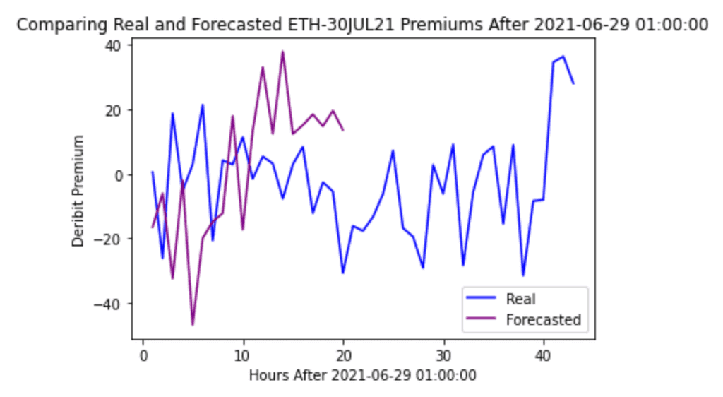
Our light blue predictions match the sharp rises and falls of the dark blue data rather well, as there is much overlap between the two. We also calculate an MSE loss of 517.76 to quantify this overlap. To evaluate our 20 forecasted premiums, we wait approximately 40 hours and compare the forecast with the actual data:
In the first 7 or so hours, the directions of the premiums in the forecast align with those in the real data. Afterwards, however, the model does not forecast the directions as accurately and seems to expect the premium to hover around 40. This suggests that the model cannot extrapolate too far into the future, which could potentially be remedied by including more than 743 hourly premiums in the initial data or increasing model complexity by including more hidden layers and/or neurons. Nevertheless, our LSTM serves as a proof-of-concept of the ability of sequential machine learning models to forecast highly volatile cryptocurrency data and thereby help us make more informed trading decisions.
